Scaling and System Design Basics: What Backend Engineers Need to Know
Introduction
Every system starts on a single server. At some point that server isn't enough — too many requests, too much data, too many concurrent users. How you respond to that problem determines whether your system survives growth or buckles under it.
Scaling is not just about adding more hardware. It's about understanding the tradeoffs between different approaches, knowing where your bottlenecks actually are, and making deliberate architectural decisions before the load arrives rather than after.
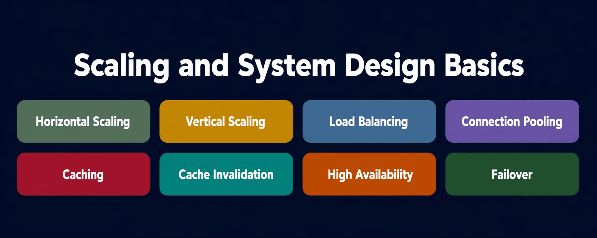
This post covers the core scaling and system design concepts that come up in every senior backend interview:
- Horizontal vs vertical scaling — the two fundamental approaches and when each applies
- Load balancing — routing traffic across servers, algorithms, health checks, and session handling
- Connection pooling — why raw connections are expensive and how pooling fixes that
- Caching — patterns, eviction policies, invalidation strategies, and the hardest problems
- High availability — what it actually means and how it's measured
- Failover — automatic vs manual, types of failover, and what can go wrong
Section 1 — Horizontal vs Vertical Scaling
🔹 Vertical Scaling (Scale Up)
Simple Explanation
Vertical scaling means making your existing server more powerful — adding more CPU cores, more RAM, faster storage. One machine, more capacity.
Analogy
You're running a restaurant with one chef. Business picks up so you get a better chef who works faster, with more skills, and more equipment. The kitchen is still one kitchen — just a more powerful one.
Mini Diagram
Before:
[Server: 4 cores, 16GB RAM, 500GB SSD]

After vertical scaling:
[Server: 32 cores, 256GB RAM, 4TB NVMe SSD]

Same single machine → more powerful
The hard ceiling
Vertical scaling has a physical limit. At some point, you can't buy a bigger machine. The most powerful single servers available have around 128–192 CPU cores and a few terabytes of RAM. Beyond that, you can't scale further — and the biggest machines are also the most expensive per unit of compute.
There's also a second problem: a single server is a single point of failure. When it goes down, everything goes down.
✅ Vertical scaling works well when:
- Your workload can't be distributed (e.g., a database that requires strict single-node consistency)
- You need a quick fix and don't have time to redesign the architecture
- The load increase is modest and within the machine's headroom
❌ Vertical scaling fails when:
- You've hit the hardware ceiling
- You need fault tolerance — one powerful machine still fails
- Cost becomes unreasonable at the high end of server specs
🔹 Horizontal Scaling (Scale Out)
Simple Explanation
Horizontal scaling means adding more machines instead of making one machine more powerful. The workload is distributed across multiple servers. Each server handles a portion of the traffic.
Analogy
Instead of hiring one super-chef, you hire ten regular chefs and give each one a section of orders. More people, more tables served. The restaurant scales by expanding the team, not by making one person superhuman.
Mini Diagram
Before:
[Server 1] ← handles all 10,000 req/sec

After horizontal scaling:
[Server 1] ← 2,500 req/sec
[Server 2] ← 2,500 req/sec
[Server 3] ← 2,500 req/sec
[Server 4] ← 2,500 req/sec
         ↑
  Load balancer distributes traffic
Why horizontal scaling dominates at scale
Horizontal scaling is theoretically unlimited — add more machines as needed. It also provides fault tolerance: if one server fails, the others continue handling traffic. Most modern cloud infrastructure (AWS Auto Scaling, Kubernetes Horizontal Pod Autoscaler) is built entirely around horizontal scaling.
The tradeoff is complexity. Distributing state across multiple machines introduces problems that don't exist on a single server: how do users maintain sessions across different servers? How do you keep data consistent across nodes? How do you route traffic intelligently?
✅ Horizontal scaling works well when:
- Your application is stateless (each request is independent)
- You need fault tolerance and high availability
- Traffic is unpredictable and you need elastic capacity
- You've outgrown what any single machine can handle
❌ Horizontal scaling is harder when:
- Your application maintains server-side session state
- Your data layer can't be sharded or distributed
- The overhead of coordinating across nodes outweighs the benefit (for some database workloads)
Stateless design is a prerequisite
For horizontal scaling to work cleanly, your application servers must be stateless — no local session data, no in-memory state that differs between servers. Any state that needs to persist between requests (user sessions, shopping carts, authentication tokens) must live in a shared store: a database, Redis, or a distributed cache. Every server can then handle any request from any user.
This is why the shift to horizontal scaling often requires an explicit "make the app stateless" refactoring before you can scale out effectively.
Section 2 — Load Balancing
🔹 Load Balancing
Simple Explanation
A load balancer sits in front of your servers and routes incoming requests across them. Its job is to prevent any single server from being overwhelmed while ensuring requests get to healthy servers. It's also the component that makes horizontal scaling transparent to clients — users hit one address, the load balancer handles the rest.
Analogy
Airport check-in. Twenty check-in desks, one queue. An attendant directs each person to an available desk. Nobody queues at a desk that's busy when others are free. If a desk closes, the attendant stops sending people there. That attendant is the load balancer.
Mini Diagram
Client requests
       ↓
  [Load Balancer]
  ↙     ↓      ↘
[S1]  [S2]  [S3]

S2 goes down → Load Balancer detects via health check
→ Routes traffic to S1 and S3 only
→ S2 removed from rotation ✓
Load Balancing Algorithms — the detail interviews test
Round Robin
The simplest algorithm. Requests are distributed evenly across all servers in sequence. Request 1 goes to S1, request 2 to S2, request 3 to S3, request 4 back to S1, and so on.
Request 1 → S1
Request 2 → S2
Request 3 → S3
Request 4 → S1 (back to start)
Works well when all servers have the same capacity and requests take roughly the same time. Falls apart when some requests are much heavier than others — a server handling expensive requests can get overloaded even while receiving "equal" traffic by count.
Weighted Round Robin
Same as round robin, but servers are assigned weights based on their capacity. A server with twice the resources gets twice as many requests.
S1: weight=1  → gets 1 request per cycle
S2: weight=2  → gets 2 requests per cycle
S3: weight=1  → gets 1 request per cycle

Cycle: S1, S2, S2, S3 → repeat
Useful when your server fleet is heterogeneous — you've added newer, more powerful servers alongside older ones and want traffic proportional to capacity.
Least Connections
Routes each new request to the server with the fewest active connections. Adapts in real time to servers that are working harder.
S1: 45 active connections
S2: 12 active connections ← new request goes here
S3: 38 active connections
Better than round robin when requests have highly variable processing times. A server handling long-running connections naturally receives fewer new ones. Most appropriate for API servers, WebSocket connections, or anything with sustained open connections.
IP Hash (Sticky Sessions)
Routes requests from the same client IP to the same server, every time. Ensures session persistence without a shared session store.
Client IP: 103.22.44.55 → always routes to S2
Client IP: 45.66.77.88  → always routes to S3
Solves the problem of server-side session state — if user data is stored in S2's memory, that user always needs to reach S2. The downside: if S2 goes down, all sessions on S2 are lost, and those users have to start fresh on a different server. It also creates uneven distribution if some IPs generate much more traffic than others.
Least Response Time
Routes to the server with the lowest combination of active connections and response time. More sophisticated than least connections — it accounts for server speed, not just load.
Random with Two Choices (Power of Two)
Pick two servers at random, route to whichever has fewer connections. Surprisingly effective — performs close to least connections with much lower overhead. Used by Nginx and several CDNs.
Health Checks
A load balancer is useless if it routes traffic to dead servers. Health checks solve this.
Passive health checks: the load balancer monitors responses. If a server returns errors (5xx) or times out repeatedly, it's marked unhealthy and removed from rotation.
Active health checks: the load balancer periodically sends its own requests (usually a dedicated /health endpoint) to each server. If the server doesn't respond with a 200 within a timeout, it's marked unhealthy.
Load Balancer → GET /health → S1 → 200 OK ✓ (healthy)
Load Balancer → GET /health → S2 → timeout ✗ (unhealthy, removed)
Load Balancer → GET /health → S3 → 200 OK ✓ (healthy)

Traffic now routes only to S1 and S3
A good /health endpoint doesn't just return 200 automatically. It checks that the application's dependencies (database connection, cache connection, downstream services) are healthy. An application that's running but can't reach its database should return 503, not 200.
Layer 4 vs Layer 7 load balancing
Layer 4 load balancers operate at the TCP/UDP level. They route based on IP address and port. Fast, minimal overhead, but no visibility into HTTP content. Can't make routing decisions based on URL paths or headers.
Layer 7 load balancers operate at the HTTP/application level. They can route based on URL path (/api to one server pool, /static to another), HTTP headers, cookies, or request body content. More flexible, slightly more overhead. Most production systems use Layer 7.
Layer 7 example (Nginx):
/api/*      → backend server pool (port 8080)
/static/*   → CDN or static file servers
/websocket  → WebSocket server pool (port 8081)
The load balancer as a single point of failure
A load balancer that's not redundant is itself a single point of failure. The standard fix: run two load balancers in active-passive configuration. One is active, the other is standby. A floating IP address (virtual IP) is shared between them. If the active load balancer fails, the virtual IP switches to the passive one in seconds.
AWS ALB, GCP Load Balancer, and Cloudflare are managed services that handle their own redundancy — you don't manage the load balancer infrastructure yourself.
✅ Use Layer 7 when:
- You need path-based or header-based routing
- You want SSL termination at the load balancer
- You need visibility into HTTP metrics per route
✅ Use Layer 4 when:
- You need maximum throughput with minimum latency
- You're routing non-HTTP traffic (databases, message brokers)
- CPU overhead of Layer 7 inspection is a concern
Interview Insight
"How do you handle session persistence without sticky sessions?" The answer is to make the application stateless. Move session data out of server memory and into a shared Redis cluster. Every server can reconstruct any user's session from Redis, so any server can handle any request. This is the right answer — sticky sessions are a workaround for stateful servers, not a solution. The solution is making the application stateless.
Section 3 — Connection Pooling
🔹 Connection Pooling
Simple Explanation
Every time your application opens a new database connection, there's overhead: TCP handshake, authentication, session initialisation, security verification. Research shows this takes 8–27ms per connection depending on the database. For an application handling 500 requests per second, creating a new connection per request adds up to seconds of cumulative overhead per second — far more than the queries themselves.
Connection pooling solves this by creating a fixed set of connections at startup and reusing them. A request borrows a connection from the pool, does its work, and returns the connection when done.
Analogy
A taxi fleet vs a ride-hailing service. A ride-hailing service dispatches a car, it does the trip, then it's available for the next request immediately — the car doesn't go back to a garage between fares. That's connection pooling. Creating a new connection per request is like buying a new car for every fare and scrapping it afterwards.
Mini Diagram
Without pooling:
Request 1 → create connection → query → close connection  (8-27ms overhead)
Request 2 → create connection → query → close connection  (8-27ms overhead)
Request 3 → create connection → query → close connection  (8-27ms overhead)

With pooling:
Pool initialised: [Conn1] [Conn2] [Conn3] [Conn4] [Conn5]

Request 1 → borrows Conn1 → query → returns Conn1  (<1ms overhead)
Request 2 → borrows Conn2 → query → returns Conn2  (<1ms overhead)
Request 3 → borrows Conn1 (now free) → query → returns Conn1
Pool size configuration — where most engineers get it wrong
Two failure modes:
Pool too small: all connections are in use. New requests queue up waiting for a connection. Under high load, the queue grows and requests time out. Throughput is throttled by the pool size.
Pool too large: each connection consumes resources on the database server (memory, CPU for idle connection maintenance). PostgreSQL uses about 5–10MB per connection. A pool of 500 connections on a small database server consumes 2.5–5GB of RAM just for connection overhead — before any data is cached.
The standard formula for PostgreSQL pool size:
pool_size = (number_of_cores * 2) + effective_spindle_countFor a 4-core server with SSDs (count as 1): pool size ≈ 9.
This is smaller than most engineers expect. The reason: database operations are I/O bound, not CPU bound. More connections than the database can actively process just queue up anyway. Fewer, busier connections are more efficient than many idle ones.
PgBouncer for PostgreSQL
PostgreSQL creates a separate OS process per connection — expensive at scale. PgBouncer is a connection pooler that sits between your application and PostgreSQL. The application maintains a large pool to PgBouncer; PgBouncer maintains a small pool to PostgreSQL.
Application servers (many): each with pool of 10 connections
         ↓ (up to 100 concurrent connections to PgBouncer)
     [PgBouncer]
         ↓ (15-20 actual connections to PostgreSQL)
     [PostgreSQL]
PgBouncer supports three modes:
Session pooling: a PgBouncer connection is held for the entire duration of a client session. Least efficient.
Transaction pooling: a connection is held only for the duration of a transaction, then returned. Most common for web applications. The application gets a connection for its transaction and releases it immediately.
Statement pooling: a connection is held only for a single statement. Fastest, but breaks anything that uses multi-statement transactions. Rarely used.
Node.js example with pg pool
const { Pool } = require('pg');

const pool = new Pool({
  host: 'localhost',
  database: 'mydb',
  user: 'postgres',
  password: 'secret',
  max: 10,            // max connections in pool
  min: 2,             // min connections kept alive
  idleTimeoutMillis: 30000,   // close idle connections after 30s
  connectionTimeoutMillis: 2000,  // fail if no connection available in 2s
});

// Usage — pool handles connection acquisition/release automatically
const result = await pool.query('SELECT * FROM users WHERE id = $1', [userId]);
MongoDB connection pooling
MongoDB's Node.js driver manages connection pooling automatically:
const { MongoClient } = require('mongodb');

const client = new MongoClient(uri, {
  maxPoolSize: 10,         // max connections in pool
  minPoolSize: 2,          // min connections to maintain
  maxIdleTimeMS: 30000,    // close idle connections after 30s
  waitQueueTimeoutMS: 2000 // fail if no connection available in 2s
});

await client.connect();
// Reuse this client across your application — don't create a new client per request
The most common MongoDB connection pool mistake: creating a new MongoClient on every request. Each client creates its own pool. Create one client at application startup and share it across all requests.
Interview Insight
"What happens when your connection pool is exhausted?" Requests queue up waiting for a free connection. If the queue timeout is hit, requests fail with a "connection timeout" error. This often shows up as cascading failures — a slow database query holds connections longer than usual, the pool exhausts, downstream requests fail, and the error rate spikes suddenly. Monitoring pool wait times alongside query times is how you catch this before it becomes an outage.
Section 4 — Caching
🔹 Caching
Simple Explanation
Caching stores the results of expensive operations — database queries, API calls, complex computations — in a faster storage layer (usually memory) so subsequent requests can be served without repeating the expensive work.
The fundamental premise: computing something once and reusing it many times is cheaper than computing it repeatedly.
Analogy
A customer asks a librarian for the five most borrowed books of the year. The librarian could go through every checkout record to compute this — or they could keep a list on their desk that they update weekly. Most queries get answered from the desk, not from a full archive search. The desk is the cache.
Cache hit vs cache miss
Cache HIT:
User requests product id=42
→ Check cache → found ✓
→ Return from cache (sub-millisecond)
→ Database not touched

Cache MISS:
User requests product id=99
→ Check cache → not found ✗
→ Query database (10-100ms)
→ Store result in cache
→ Return to user
→ Next request for id=99 → cache hit ✓
Cache hit rate is the percentage of requests served from cache. A 95% hit rate means only 5% of requests reach the database. If your cache hit rate is low, you're paying the caching overhead without getting the benefit.
Caching Patterns — what interviewers really want to know
Cache-Aside (Lazy Loading)
The application checks the cache first. On a miss, it reads from the database, stores the result in the cache, and returns it. The cache is populated on demand.
async function getUser(userId) {
  // Check cache first
  const cached = await redis.get(`user:${userId}`);
  if (cached) return JSON.parse(cached);

  // Miss — fetch from database
  const user = await db.query('SELECT * FROM users WHERE id = $1', [userId]);

  // Store in cache for next time
  await redis.setex(`user:${userId}`, 3600, JSON.stringify(user)); // TTL: 1 hour

  return user;
}
The cache only contains data that's actually been requested. No wasted memory on data nobody asks for. The downside: the first request after a cache miss is always slow.
Write-Through
Every write to the database also updates the cache simultaneously. The cache is always in sync.
async function updateUser(userId, data) {
  // Write to database
  await db.query('UPDATE users SET name=$1 WHERE id=$2', [data.name, userId]);

  // Immediately update cache
  await redis.setex(`user:${userId}`, 3600, JSON.stringify(data));
}
The cache never serves stale data. But every write now has extra latency (the cache write). And you're caching data that may not be read again, wasting memory.
Write-Behind (Write-Back)
The application writes to the cache first and returns immediately. The cache asynchronously flushes writes to the database in batches.
User updates profile
→ Write to cache (fast, returns immediately)
→ Cache queues write to database
→ Database updated asynchronously (100ms later)
Fastest write performance. But if the cache crashes before the write flushes to the database, data is lost. Used for high-write scenarios where occasional data loss is acceptable (analytics counters, view counts, etc.).
Read-Through
Similar to cache-aside but the cache handles the database read itself. The application only ever talks to the cache — the cache fetches from the database on a miss. Less common in practice; most implementations use cache-aside at the application layer.
Cache Eviction Policies
When the cache fills up, something has to be removed. The eviction policy determines what.
LRU (Least Recently Used)
Evicts the item that hasn't been accessed for the longest time. The assumption: recently accessed items are more likely to be accessed again. This is the default Redis eviction policy and the most commonly correct choice.
Cache state:
item A: last accessed 5 min ago
item B: last accessed 1 min ago
item C: last accessed 30 sec ago

Cache full → new item arrives → evict item A (least recently used)
Cache full → new item arrives → evict item A (least recently used)
LFU (Least Frequently Used)
Evicts the item accessed the fewest times overall. Keeps items that are consistently popular, even if they haven't been accessed very recently.
Better than LRU for stable, predictable access patterns. Worse for access patterns where popularity shifts over time — a trending item that was unpopular yesterday gets evicted by stale popular items.
TTL (Time to Live)
Items expire after a fixed duration, regardless of access frequency. The cache stays fresh automatically.
await redis.setex('product:99', 300, JSON.stringify(product)); // expires in 300 secondsTTL is not a full eviction policy — it works alongside LRU or LFU. Items expire on their TTL, and if the cache fills up before TTLs expire, the underlying eviction policy (LRU/LFU) determines what gets removed first.
FIFO (First In, First Out)
Evicts the oldest item regardless of access frequency or recency. Simple to implement, rarely the right choice — it discards popular old items just because they were cached first.
Cache Invalidation — the hardest problem
Phil Karlton famously said there are only two hard problems in computer science: cache invalidation and naming things.
Cache invalidation is the problem of ensuring cached data is removed or updated when the underlying data changes. If you don't invalidate stale cache entries, users see outdated data. If you invalidate too aggressively, you defeat the purpose of caching.
TTL-based invalidation
The simplest approach: set a TTL on every cached item. After the TTL expires, the next request fetches fresh data.
The downside: staleness is bounded but non-zero. For a 5-minute TTL, users may see data that's up to 5 minutes old. For many use cases (product listings, blog posts, dashboards) this is fine. For others (account balances, inventory counts) it's not.
Event-driven invalidation
When data changes in the database, an event triggers cache invalidation. The cache entry is deleted or updated immediately.
async function updateProduct(productId, data) {
  // Update database
  await db.query('UPDATE products SET price=$1 WHERE id=$2', [data.price, productId]);

  // Immediately invalidate cache
  await redis.del(`product:${productId}`);

  // Next request for this product will miss cache → fetch fresh data
}
More complex but more accurate. The cache and database stay in sync. The risk: if the invalidation fails (Redis is temporarily unavailable), the cache serves stale data until the TTL expires. Always set a TTL as a fallback even when using event-driven invalidation.
Cache stampede (thundering herd)
When a popular cache entry expires, many requests arrive simultaneously, all find a cache miss, and all hit the database at once. If you have 10,000 req/sec for a product page and the cache expires, all 10,000 requests may simultaneously query the database.
Prevention strategies:
Mutex lock: the first request to miss the cache acquires a lock and fetches from the database. All other requests wait. When the first request populates the cache and releases the lock, the others serve from cache.
async function getProductWithLock(productId) {
  const cached = await redis.get(`product:${productId}`);
  if (cached) return JSON.parse(cached);

  const lockKey = `lock:product:${productId}`;
  const lockAcquired = await redis.set(lockKey, '1', 'NX', 'EX', 5); // 5s lock TTL

  if (lockAcquired) {
    const data = await db.query('SELECT * FROM products WHERE id = $1', [productId]);
    await redis.setex(`product:${productId}`, 3600, JSON.stringify(data));
    await redis.del(lockKey);
    return data;
  } else {
    // Wait briefly and retry — lock holder is populating the cache
    await new Promise(r => setTimeout(r, 50));
    return getProductWithLock(productId);
  }
}
Probabilistic early expiration: before the TTL expires, randomly start refreshing it early based on how close to expiry it is. The earlier a cache entry is in its TTL, the less likely it gets refreshed early. This smooths cache misses over time instead of batching them at expiry.
Staggered TTLs: add random jitter to TTLs so entries for similar data don't all expire at the same moment.
const ttl = 3600 + Math.floor(Math.random() * 300); // 60–65 minutes, random
await redis.setex(`product:${productId}`, ttl, JSON.stringify(data));
Multi-Layer Caching
In production systems, caching is typically layered. Each layer is faster but smaller than the one below it.
Browser cache (client-side)
         ↓ on miss
CDN (edge cache — geographically close to user)
         ↓ on miss
Application cache (Redis, Memcached — in-memory, shared)
         ↓ on miss
Database query cache (optional, built into the database)
         ↓ on miss
Database (source of truth)
Each layer serves the request if it can, only falling through to the next if it can't. A request for a static asset (image, CSS, JS) might be served entirely from the browser cache or CDN — the origin server never sees it.
Redis vs Memcached
Both are in-memory data stores used for caching. Redis is the standard choice for most systems today because it supports:
- Richer data structures (lists, sets, sorted sets, hashes) beyond just key-value strings
- Persistence (can write to disk, so data survives a restart)
- Pub/sub for event-driven cache invalidation
- Atomic operations for things like rate limiting and distributed locks
- Cluster mode for horizontal scaling
Memcached is simpler, slightly faster for pure key-value string caching at extreme scale, and uses less memory per item. It's rarely the right choice for a new system.
Interview Insight
"What's the hardest part of caching?" Cache invalidation. Follow up with: "How do you handle it?" The answer should cover TTL as a baseline, event-driven invalidation for time-sensitive data, and the cache stampede problem with at least one mitigation strategy. Interviewers want to know you understand that caching introduces consistency problems, not just performance benefits.
Section 5 — High Availability
🔹 High Availability (HA)
Simple Explanation
High availability is the property of a system that continues operating correctly even when individual components fail. It's measured as a percentage of uptime over time.
99%   uptime → 87.6 hours downtime per year   (not HA)
99.9%         →  8.76 hours downtime per year
99.99%        →  52.6 minutes downtime per year
99.999%       →  5.26 minutes downtime per year  ("five nines")
The gap between 99% and 99.999% is enormous. Going from 99.9% to 99.99% requires eliminating roughly 8 hours of downtime per year — that's the difference between "we had an incident" and "we had zero incidents."
What HA actually requires
No single point of failure. Every component in the system must have a redundant backup. If any component fails without a backup, that component is a single point of failure and its downtime is your downtime.
Components that need redundancy:
→ Application servers (horizontal scaling provides this)
→ Load balancers (active-passive pair)
→ Databases (primary + replica with automatic failover)
→ Caches (Redis cluster or Sentinel for HA)
→ Message queues (clustered brokers)
→ DNS (multiple nameservers)
→ Network (multiple network paths)
Redundancy vs fault tolerance
Redundancy means having a backup. Fault tolerance means the system continues operating correctly without human intervention when the backup activates. A system can have redundancy but not fault tolerance — if switching to the backup requires a manual step, you have redundancy but not automated fault tolerance.
SLAs, SLOs, and SLIs
High availability commitments are formalised as:
SLI (Service Level Indicator): a metric you measure (e.g., request success rate, latency p99).
SLO (Service Level Objective): the target you set (e.g., 99.9% of requests succeed, p99 latency < 200ms).
SLA (Service Level Agreement): a contractual commitment with consequences if the SLO is not met (e.g., credits to customers if uptime drops below 99.9%).
In interviews, knowing these terms and their relationship shows you understand how HA is managed operationally, not just architecturally.
Section 6 — Failover
🔹 Failover
Simple Explanation
Failover is the process of switching from a failed primary component to a backup. The goal is to minimise the duration of the outage — ideally making the failure invisible to users.
Automatic vs manual failover
Automatic failover: the system detects failure and switches to backup without human intervention. Faster, but requires confidence that the detection is accurate. False positives (detecting failure when the primary is actually fine) can cause unnecessary failovers, which introduce their own disruption.
Manual failover: a human decides when to switch. Slower (minutes to hours depending on the incident response), but gives humans a chance to verify the failure before acting.
Most production databases use automatic failover for regional failures (one data centre goes down) and manual failover for planned maintenance or cross-region failovers.
Types of failover
Active-Passive: one primary handles all traffic. The passive backup sits idle, continuously replicating from the primary but not serving requests. When the primary fails, the passive takes over.
Normal:   Client → [Primary] → serves all traffic
                   [Passive] → replicating, idle

Failure:  Primary fails
          [Passive] → promoted to primary ✓
Client → [New Primary] → serves traffic
Active-Active: multiple nodes are all active simultaneously. If one fails, traffic is redistributed among the remaining active nodes. No promotion step required — the load balancer simply routes away from the failed node.
Normal:   Client → [LB] → [Node A] + [Node B] + [Node C]

Node B fails:
          Client → [LB] → [Node A] + [Node C]
          (traffic redistributed automatically)
Active-active is preferred for application servers behind a load balancer. For databases, it requires either multi-leader replication (complex) or a shared storage layer.
Failover risks and what can go wrong
Split-brain during failover: the primary is slow but not dead. The backup gets promoted. Now both are accepting writes. (Covered in detail in the previous article — prevented by quorum and fencing.)
Data loss during failover: if replication is async, writes that reached the primary but not the replica are lost when the replica is promoted. The amount of data loss is bounded by replication lag at the time of failure.
Failover takes longer than expected: automated failover detection has a detection window. PostgreSQL with Patroni has a default detection window of 10–30 seconds. During that window, the database is unavailable. Applications must implement retry logic for this period.
Cascading failures: failover increases load on remaining nodes. If they were already near capacity, the failover of one node may overload the others, causing them to fail in turn. This is why capacity planning includes headroom for N-1 nodes to handle full traffic.
Database failover in practice
PostgreSQL with Patroni:
Normal: [Primary PostgreSQL] ← Patroni holds leader key in etcd
        [Replica 1] [Replica 2] → replicating async

Primary fails:
→ Patroni detects: leader key in etcd not renewed
→ Replicas run election (Raft-inspired)
→ Replica 1 promoted to primary (most up-to-date log)
→ Replica 2 switches to replicating from Replica 1
→ Application connection string points to Patroni-managed VIP
→ VIP switches to new primary → apps reconnect automatically
→ Total failover time: 10–30 seconds typical
MongoDB automatic failover:
Normal: [Primary] + [Secondary 1] + [Secondary 2]

Primary fails:
→ Secondaries detect missing heartbeat (10 second timeout)
→ Election starts: Secondary 1 requests votes
→ Secondary 2 votes yes
→ Secondary 1 becomes new primary (majority: 2/3)
→ Drivers detect primary change via replica set monitoring
→ Write operations automatically route to new primary
→ Total failover time: 10–30 seconds typical
Interview Insight
"What's the difference between high availability and disaster recovery?" HA handles component-level failures (a single server, a single database node) automatically, with minimal downtime (seconds to minutes). Disaster recovery handles region-level failures (an entire data centre goes down) and typically involves more downtime (minutes to hours), restoring from backups or failing over to a secondary region. HA is for the everyday; DR is for the catastrophic.
Section 7 — Putting It All Together
These concepts don't operate independently. Here's how a typical production architecture stacks them:
User request arrives
         ↓
[DNS] → resolves to load balancer VIP
         ↓
[Load Balancer] (active-passive pair for HA)
→ health checks confirm which app servers are alive
→ routes via least connections or round robin
         ↓
[Application Server Pool] (horizontal scaling)
→ stateless: any server can handle any request
→ check [Cache (Redis)] for data first
   → cache hit: return immediately ✓
   → cache miss: query database, populate cache, return
         ↓ (on cache miss)
[Connection Pool (PgBouncer)] → manages DB connections
         ↓
[Database Primary] (PostgreSQL or MongoDB)
→ async replication to [Read Replicas]
→ Patroni/Replica Set handles automatic failover

Failure scenarios:
→ App server dies: load balancer routes away (health check)
→ Cache dies: requests fall through to database (degraded but functional)
→ Database primary dies: automatic failover in 10-30s, apps retry
→ Entire AZ goes down: traffic fails over to secondary region (HA + DR)
How These Concepts Appear in Real Systems
AWS
Horizontal scaling via Auto Scaling Groups — adds EC2 instances when CPU exceeds a threshold, removes them when load drops. Application Load Balancer (Layer 7) routes traffic across instances. ElastiCache (Redis) for caching. RDS with Multi-AZ for automatic database failover. Connection pooling via RDS Proxy.
Kubernetes
Horizontal Pod Autoscaler scales pod count based on CPU/memory metrics or custom metrics. Services provide load balancing across pods (Layer 4 by default, Layer 7 with Ingress controllers). Redis deployed as a StatefulSet for HA caching. PostgreSQL deployed via operators (CloudNativePG, Zalando PostgreSQL Operator) with automatic failover.
Netflix
Horizontal scaling across thousands of EC2 instances. Chaos Monkey deliberately kills random instances to verify that the system handles failures automatically. EVCache (a distributed Memcached wrapper) for caching at massive scale. Zuul as their API gateway / load balancer. Hystrix (now mostly superseded) for circuit breaking — preventing a slow service from cascading failures to callers.
Cloudflare
Anycast routing — the same IP address is announced from data centres worldwide. Users are automatically routed to the nearest data centre. DDoS protection and rate limiting at the load balancer layer. Edge caching serves static and cacheable content globally without hitting origin servers.
Conclusion
Scaling is a series of tradeoffs, not a single decision. Here's the mental model to carry forward:
- Vertical scaling is the quick fix with a hard ceiling. Use it for databases that can't be distributed, or as a first step before architectural changes.
- Horizontal scaling is the long-term path. Requires stateless application design. Enable it early, before you need it.
- Load balancing distributes traffic and removes single points of failure. Use least connections for variable workloads, round robin for uniform ones. Always build active health checks. Make the load balancer itself redundant.
- Connection pooling eliminates the overhead of creating database connections per request. Size your pool based on database capacity, not application concurrency. Use PgBouncer for PostgreSQL at scale.
- Caching trades data freshness for speed. Cache-aside is the most common pattern. Set TTLs on everything. Plan your invalidation strategy before you need it. Handle cache stampedes.
- High availability means no single point of failure plus automated failover. Measure it as uptime percentage. Understand the difference between redundancy and fault tolerance.
- Failover works automatically in well-designed systems. Active-active is better than active-passive for application servers. Database failover takes 10–30 seconds in modern systems — applications must retry during this window.
The engineers who design systems that handle failures gracefully are not the ones who prevented all failures. They're the ones who assumed failures would happen and built the system to continue anyway.